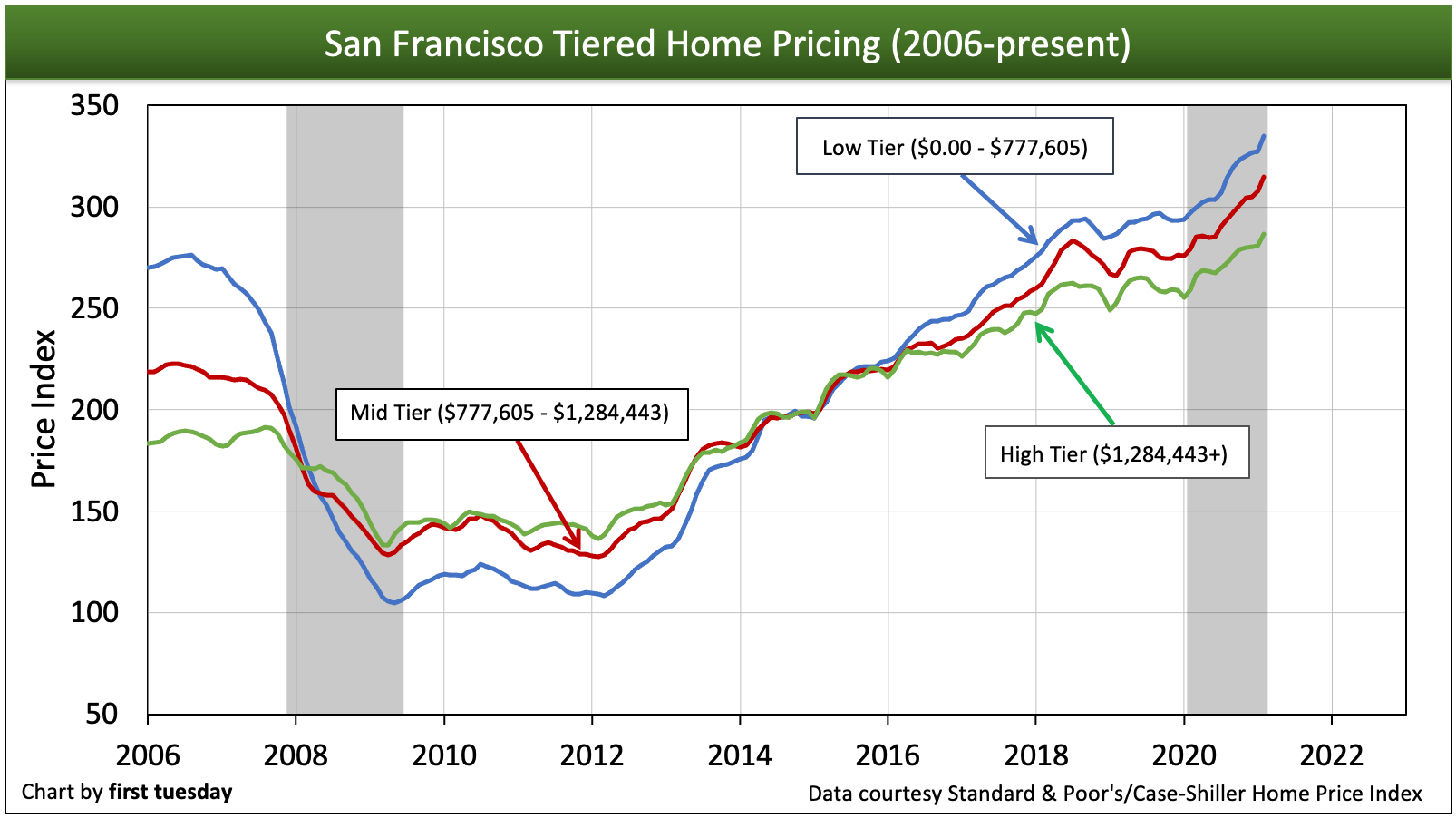
Home prices continued to rise rapidly in all tiers across Los Angeles, San Diego and San Francisco during February 2021. The statewide average for low- mid- and high-tier prices was 14% higher than a year earlier. These significant price jumps continue to gain momentum heading into the spring peak home sale season, despite the ongoing recession.
Starting in Q1 2020, job losses, economic volatility and shelter-in-place orders caused home sales volume to decline, picking up in the second half of the year. Typically, home prices fall within a few months of a consistent drop in sales volume. But historically low interest rates provided a boost for buyer purchasing power, which, along with competition for a dwindling inventory of homes for sale, inflated home prices and sales volume in 2020, continuing in 2021.
Looking ahead, the future trend for home prices in 2022 will be down, the result of historic job losses and high levels of 90+ day mortgage delinquencies, which will lead to a wave of distressed sales when the foreclosure moratorium lifts, currently scheduled to occur in mid-2021. Once foreclosures return, home prices are expected to fall, bottoming around 2023.
The housing market’s performance in the next couple of years will depend on the timing and extent of any additional stimulus and/or extensions of the foreclosure and eviction moratoriums. But the most impact will come from job creation, whether it be through government-sponsored programs or jobs returning organically over the next several years. Either way, the recovery of jobs is essential to returning some stability to the housing market.
The above charts track sales price fluctuations of single family residence (SFR) resales in California’s three largest cities. Each city’s sales prices are organized by price tier, giving a clearer picture of price movement in each price range within the market.
To understand the “big picture” of the disparity between low-, middle-, and high-tier sales fluctuations, look to the Standard & Poor’s/Case-Shiller home price index as the authority. The index is an invaluable source of information and price comparisons for California’s three major cities and the state as a whole.
The below charts track changes in specific tiers according to the Case-Shiller home price index, displaying how different ranges of house prices in the market perform in comparison to one another. Portrayals of pricing in California take many forms. The index figure is particularly useful as it displays relative price movement rather than a misleading dollar amount which actually fits no single property.
Unlike many media sources, first tuesday shuns the simplistic median price approach. That approach tracks all home prices as a single tier by assigning them one average price. This one-price-fits-all dollar amount looks good on paper, but means nothing in the real world since it is a mathematical abstraction. Neither the actual nor adjusted median price represents the price of any single property. For the vast majority of properties sold or for sale, the median is a mathematical distortion.
Brokers seeking the actual value of a specific property would do well to remember that there is no such thing as a “median priced home” — you simply cannot find it. Median price is a statistical point which fails to work in the analysis of any price-tier analysis of properties, much less an individual property.
To determine how real estate will actually behave in the future, you cannot compare the price of a low-tier property with that of a high-tier property. Properties in different tiers move in price for very different reasons. Although the market tends to move in the same direction over time, the percentage of movement can vary greatly from tier to tier.
The best way to initially evaluate a property and set its price is to study comparable property values in the same demographic location (same house, same tract). Other ways to set the ceiling price include:
- cost per square foot (replacement cost); and
- income analysis methods.
Return to sanity
Price persistence and illiquidity are the two factors Economist John Krainer uses to explain price movement:
Price persistence is the tendency of listed prices in owner-occupied real estate to resist change, staying high even when the market for resale homes has dropped, a condition more commonly called sticky prices, downward price rigidity or the money illusion.
Prices in California have suffered from sticky prices in 2017 and 2018. During these years, home sales volume has remained flat-to-down and interest rates have steadily increased. And yet, home prices remained high for so long for two reasons:
- the lack of residential construction, particularly in the low tier where homebuyers are most eager to enter the market; and
- the steady jobs recovery across California, allowing homebuyer incomes to (almost) keep pace with home prices.
However, the Federal Reserve (the Fed) continues to increase their benchmark interest rate going into 2019, and the resulting loss in buyer purchasing power are causing home prices to finally begin to cool.
Search frictions and debt overload hindrance
The reluctance of prices to adjust quickly to real financial conditions in the real estate market is due to one particular cause; the difficulty of finding a property through a gatekeeper such as a broker, agent or builder, and then agreeing to an appropriate price, called search frictions.
In the hunt for a home, these search frictions make it far more difficult for properties to change hands and prices to be negotiated at current market rates. This prevents deals from being made when making a deal is what everyone has in mind. Thus, these frictions hinder the speedy resolution of a financial crisis, and work to the future detriment of the multiple listing service (MLS) environment.
Seller’s agents could be far more helpful by figuring out what it is they are selling, the due diligence rub that they so far are finding difficult to act on, then prepare a humble package about the conditions of the property improvements (TDS/NHD and reports), its title, its operating expenses, neighborhood statistics and the like for the buyer and the buyer’s agent to be able to make fast decisions.
If only we could stick to a cash price
Japan’s financial crisis of 1990 included a collapse in both commercial and residential property values. Income property prices were especially volatile throughout the collapse, ultimately falling faster and deeper than owner-occupied residential prices, but bottoming sooner since investors are more rational. Owner-occupied residential real estate, which had a much higher variety of pricing and a greater burden of debt, also eventually fell catastrophically, but less dramatically.
The difference in price movement is because income-producing real estate is more easily evaluated (by capitalization rates (cap rates), income flow, and replacement costs) and typically less burdened by high loan-to-value (LTV) debt ratios so equity remains to be worked with. These conditions of ownership make it easier for buyers and sellers to agree upon an appropriate price; thus, providing the owner with the ability to cash out — greater liquidity.
The relative ease of income property evaluation makes that part of the real estate market a more exciting and less predictable field, as cap rates can change dramatically, altering market values in a moment. Conversely, owner-occupied residential property moves slowly and steadily with sticky pricing, sellers not reacting to the recessionary market forces existing at the time. The historical reality of market implosion.
Readers should remember that real estate pricing often fails to correspond to objective reality. The discrepancy between the prices that homeowners set and the prices homes actually garner in the market is attributable to the human factor. Outrageous bubbles become more outrageous, and collapses become more devastating, due to a common set of irrational beliefs about market behavior. The most dramatic example of market fallibility took place in the very recent past — our Great Recession.
Charts are updated monthly. There is a two-month lag in reported data.
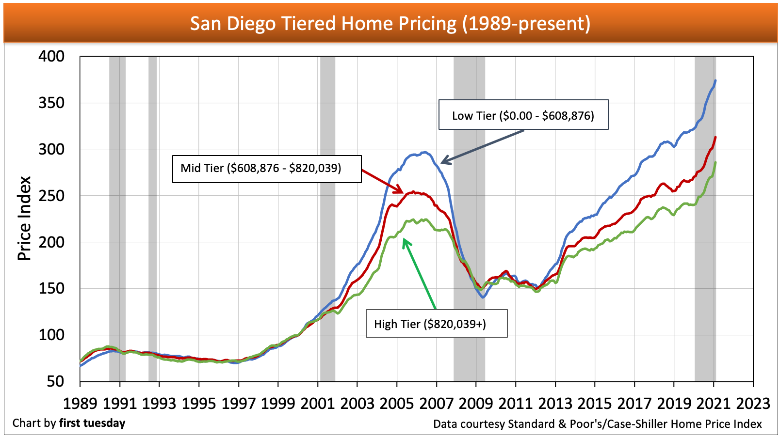
Chart update 04/27/21
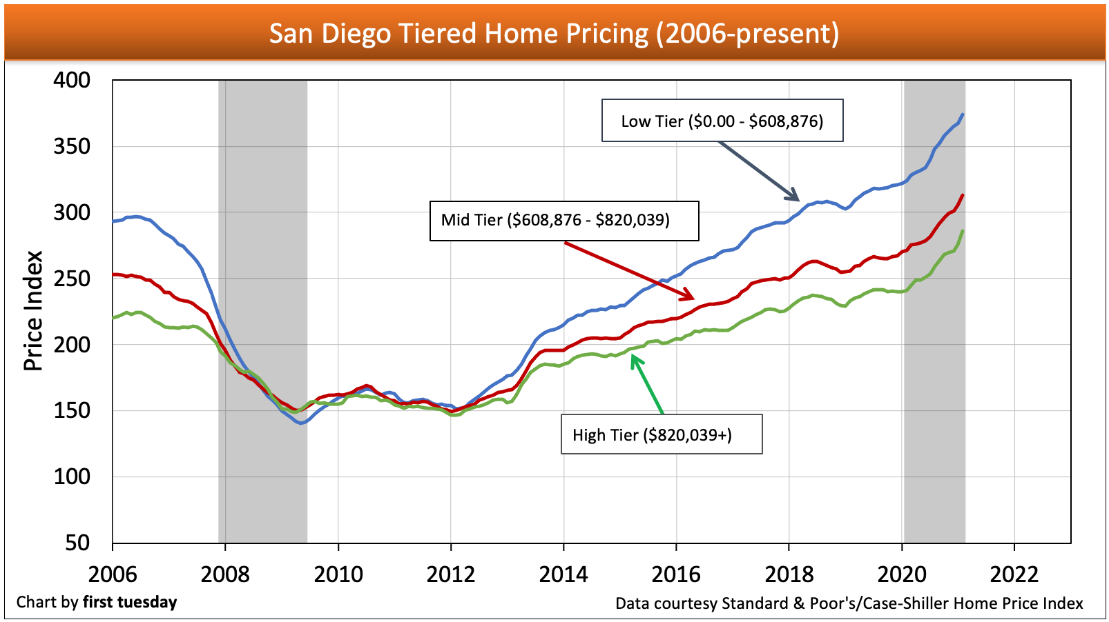
Chart update 04/27/21
| Feb 2021 | Jan 2021 | Feb 2020 | Annual Change | |
| Low Tier | 374 | 367 | 324 | +16% |
| Mid Tier | 313 | 306 | 271 | +15% |
High Tier | 286 | 276 | 241 | +19% |
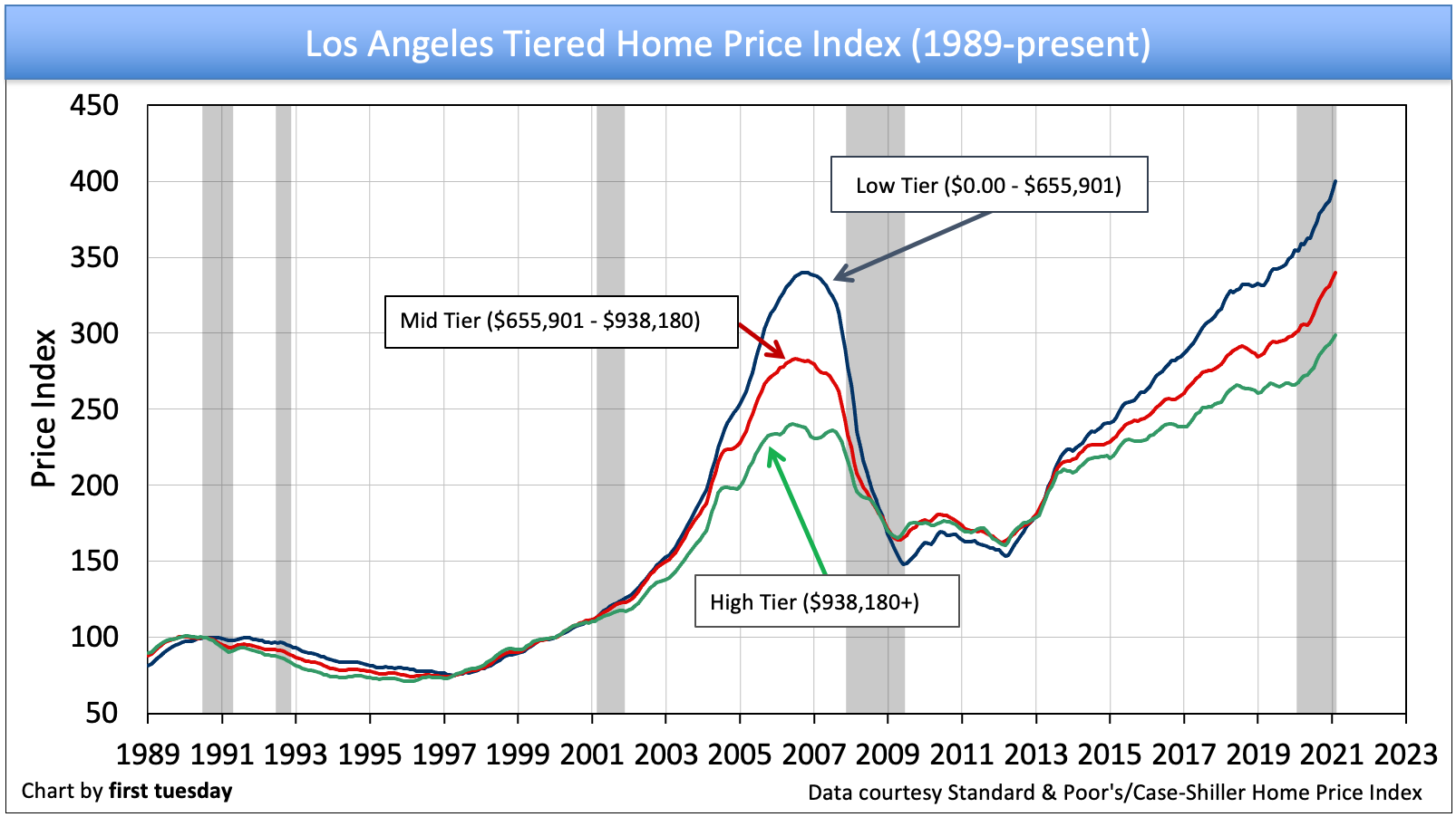
Chart update 04/27/21
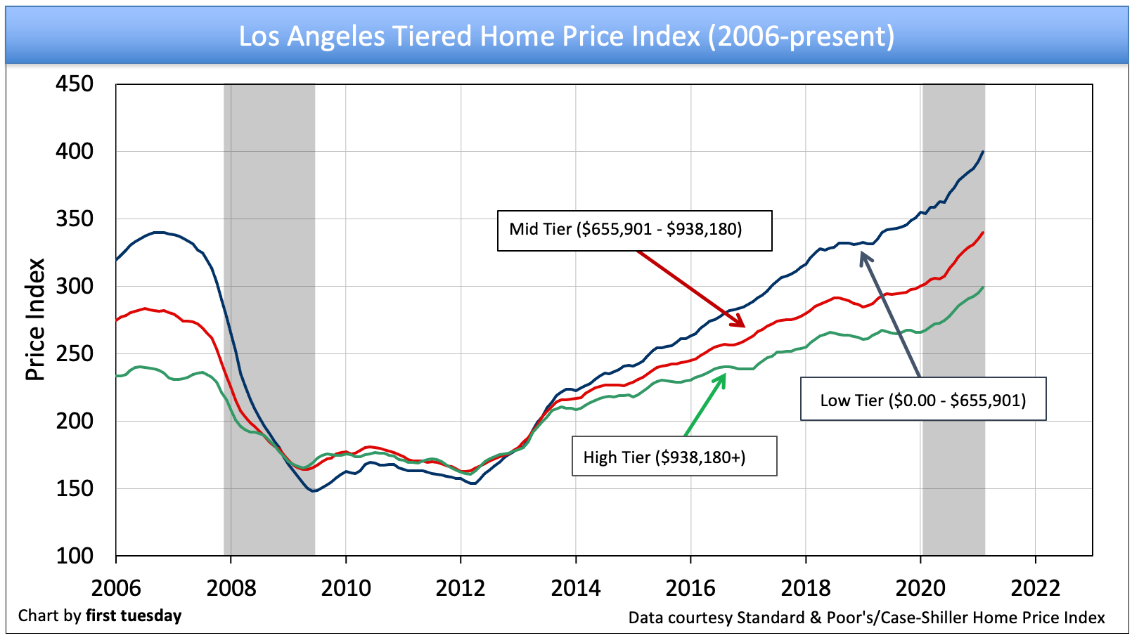
Chart update 04/27/21
| Feb 2021 | Jan 2021 | Feb 2020 | Annual Change | |
| Low Tier | 400 | 393 | 354 | +13% |
| Mid Tier | 340 | 335 | 302 | +13% |
High Tier | 299 | 295 | 268 | +12% |
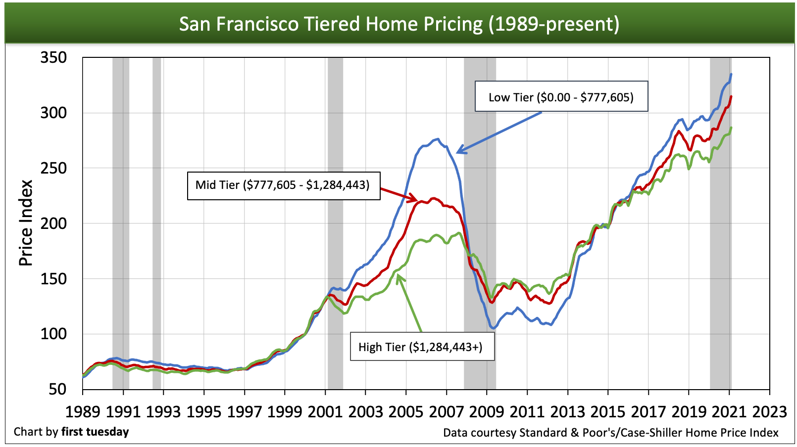
Chart update 04/27/21